Calculus III 12.01 Vector-Valued Functions

Previous	Calculus III 11 Vectors and Spacial Geometry
Next	Calculus III 12.02 Differentiation and Integration for Vector-Valued Functions

12.1 Vector-Valued Functions

• Analyze and sketch a three dimensional curve given by a vector-valued function.
• Extend limits and continuity to vector-valued functions.

Three Dimensional Curves and Vector-Valued Functions

In Section 10.2 a plane curve is defined as two ordered pairs, \((f(t),g(t))\), together with their defining parametric equations

\(x=f(t) \text{, and } y=g(t)\)

where \(f\) and \(g\) are continuous functions for \(t\) on an interval \(I\). This definition can be extended to three dimensions with three ordered pairs, \((f(t),g(t),h(t))\), together with their defining parametric equations

\(x=f(t) \text{, } y=g(t) \text{, and } z=h(t)\)

where \(f\), \(g\), and \(h\) are continuous functions for \(t\) on an interval \(I\).

Describing three dimensional curves requires a new function, called a vector-valued function which maps real numbers to vectors.

Definition 12.1.1 Vector-Valued Functions

A function with the form

\( \textbf{r}(t)=f(t)\textbf{i}+g(t)\textbf{j}\:\:\:\:\)Two-Dimensions

or

\( \textbf{r}(t)=f(t)\textbf{i}+g(t)\textbf{j}+h(t)\textbf{k}\:\:\:\:\)Three-Dimensions

is a vector-valued function, where the component functions where \(f\), \(g\), and \(h\) are real-valued functions for the parameter \(t\). Vector-valued functions are sometimes denoted as

\( \textbf{r}(t)= \langle f(t),g(t)\rangle\:\:\:\:\)Two-Dimensions

or

\( \textbf{r}(t)= \langle f(t),g(t),h(t)\rangle.\:\:\:\:\)Three-Dimensions

Where \( \textbf{r}(t)\) is a vector and the functions, \(f\), \(g\), and \(h\), produce real numbers for any \(t\).

Curve \(C\) is traced out by the terminal points along the vector \(\textbf{r}(t)\) Figure 12.1.1

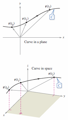
Technically, a curve is described by the points along it and the defining parametric equations. Two different curves can have the same graph. For instance, the following curves \(\textbf{r}(t)=\sin t\textbf{i}+ \cos t\textbf{j} \) and \(\textbf{r}(t)=\sin t^{2}\textbf{i}+ \cos t^{2}\textbf{j} \) have the unit circle for their graph. But the curves are traced differently. Vector-valued functions serve dual roles in describing curves. By letting the parameter \(t\) represent time, the vector-valued function can describe motion along a curve. In the more general case, the vector-valued function can trace the curve's graph. In both cases the terminal point for the position vector \(\textbf{r}(t)\) coincides with the point \((x,y)\) or \((x,y,z)\) on the curve given by the parametric equations, as shown in Figure 12.1.1. The arrowhead on the curve indicates the curve’s orientation by pointing in the direction where \(t\) increases in value. Unless stated otherwise, the domain for a vector-valued function is where the domains for the component functions \(f\), \(g\), and \(h\) intersect. For instance, the domain for \(\textbf{r}(t)=\ln t \textbf{i} + \sqrt{1-t}\textbf{j}+t\textbf{k}\) is the interval \((0,1]\).

Example 12.1.1 Sketching a Two-Dimensional Curve

The ellipse is traced clockwise as \(t\) increases from 0 to \(2\pi\). Figure 12.1.2

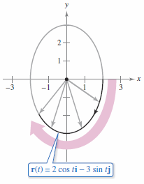
Sketch the plane curve represented by the vector-valued function \( \textbf{r}(t)=2 \cos t \textbf{i} -3 \sin t\textbf{j},\: 0 \leqslant t \leqslant 2 \pi \:\:\:\:\)Vector-valued function Solution The vector \( \textbf{r}(t)\) yields the parametric equations \(x=2 \cos t \text{ and } y= -3 \sin t\). Solving for \( \cos t \) and \( \sin t \) and using the identity \(\cos^{2}t+\sin^{2}t=1\) produces the cartesian equation $$ \frac{x^{2}}{2^{2}}+ \frac{y^{2}}{3^{2}}=1.\:\:\:\: \color{red}{ \text{ Cartesian equation}} $$ The resulting clockwise ellipse is shown in Figure 12.1.2. By clockwise means as \(t\) increases from 0 to \(2\pi\), the position vector \(r(t)\) moves clockwise, and its terminal point traces the ellipse.

Example 12.1.2 Sketching a Three-Dimensional Curve

As \(t\) increases from 0 to \(4\pi\), two spirals are traced on the helix. Figure 12.1.3

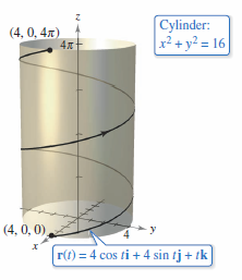
Sketch the three-dimensional curve represented by the vector-valued function \(\textbf{r}(t)=4 \cos t\textbf{i} + 4 \sin t \textbf{j} + t \textbf{k}, \: 0 \leqslant t \leqslant 4 \pi. \:\:\:\:\)Vector-valued function Solution The first two parametric equations \(x=4 \cos t\) and \(y=4 \sin t \) yield \(x^{2}+y^{2} = 16. \:\:\:\: \color{red}{ \text{ Cartesian equation}} \) The curve lies on a right cylinder with radius 4, centered about the \(z\)-axis. Use the third parametric equation \(z=t\) to locate the curve on the cylinder, as shown in Figure 12.1.3. As \(t\) increases from 0 to \(4\pi\) the point \((x,y,z)\) spirals up the cylinder to produce a single helix.

Example 12.1.3 Describe a Two-Dimensional Graph as a Vector-Valued Function

There are many ways to parametrize this graph. One way is to let \(x=t\). Figure 12.1.4

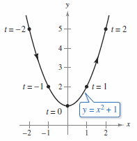
Describe the parabola \(y=x^{2}+1 \) as, shown in Figure 12.1.4, as a vector-valued function. Solution The first step is finding the parametric equations. There are many options for \(t\). The simplest is to let \(x=t\). Then \(y=t^{2}+1\). This produces \(\textbf{r}(t)=t\textbf{i}+(t^{2}+1)\textbf{j} \:\:\:\:\)Vector-valued function Note in Figure 12.1.4 the graph is traced from left to right. Had \(x=-t\) been chosen, the curve would have traced from right to left.

Example 12.1.4 Describe a Three-Dimensional Graph as a Vector-Valued Function

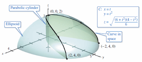
Sketch the three-dimentional curve \(C\) described by the semi-ellipsoid

$$ \frac{x^{2}}{12}+\frac{y^{2}}{24}+\frac{z^{2}}{4}=1, \:\: z \geqslant 0 $$

intersecting the parabolic cylinder \(y=x^{2}\), as shown in Figure 12.1.5. Then find a vector-valued function that describes the graph.
Solution The simplest choice for a parameter is to let \(x=t\) from the semi-ellipsoid equation. Applying this to the cylinder equation produces

\( y=x^{2} \rightarrow y=t^{2}. \)

Solving for \(z\) produces

$$ \frac{z^{2}}{4} = 1 -\frac{x^{2}}{12}-\frac{y^{2}}{24}=1 -\frac{t^{2}}{12}-\frac{t^{4}}{24}= \frac{24-2t^{2}-t^{4}}{24}=\frac{(6+t^{2})(4-t^{2})}{24}. $$

Because the curve lies above the \(xy\)-plane a positive square root for \(z\) can be chosen to produce the parametric equation

$$x=t, \: y=t^{2} \text{, and } z = \sqrt{\frac{(6+t^{2})(4-t^{2})}{6} }.$$

The resulting vector-valued function is

$$\textbf{r}(t)= t\textbf{i}+t^{2}\textbf{j}+ \sqrt{\frac{(6+t^{2})(4-t^{2})}{6} }\textbf{k}, \: -2 \leqslant t \leqslant 2.\:\:\:\:\color{red}{ \text{ Vector-valued function }}$$

Note the \( \textbf{k} \) component restricts the range to \( -2 \leqslant t \leqslant 2 \). The curve starts at (-2,4,0) and traces to (2,4,0) as \(t\) increases from -2 to 2, as shown in Figure 12.1.5.

The curve \(C\) is the intersection between a semi-ellipsoid and a parabolic cylinder.
Figure 12.1.5

Limits and Continuity

Vector-valued and real-valued functions share many algebraic properties. For example, vector-valued functions can be added, subtracted, multiplied by a scalar, differentiated, and have a limit just as real-valued functions do. This is done by extending the definitions on a component-by-component basis.

\( \textbf{r}_{1}(t) + \textbf{r}_{2}(t) \)	\(= \left[ f_{1}(t)\textbf{i} + g_{1}(t)\textbf{j}\right] + \left[ f_{2}(t)\textbf{i} + g_{2}(t)\textbf{j}\right] \:\:\:\: \)	Sum
	\(= \left[ f_{1}(t) + f_{2}(t) \right]\textbf{i} + \left[ g_{1}(t) + g_{2}(t)\right]\textbf{j} \)
\( \textbf{r}_{1}(t) - \textbf{r}_{2}(t) \)	\(= \left[ f_{1}(t)\textbf{i} + g_{1}(t)\textbf{j}\right] - \left[ f_{2}(t)\textbf{i} + g_{2}(t)\textbf{j}\right] \:\:\:\:\)	Difference
	\(= \left[ f_{1}(t) - f_{2}(t) \right]\textbf{i} + \left[ g_{1}(t) - g_{2}(t)\right]\textbf{j} \)
\( c\textbf{r}(t) \)	\(= c\left[ f_{1}(t)\textbf{i} + g_{1}(t)\textbf{j}\right] \:\:\:\:\)	Scalar Multiplication and Distribution
	\(= c f_{1}(t)\textbf{i} - cg_{1}(t) \textbf{j} \)
$$ \frac{ \textbf{r}(t)}{c} $$	$$= \frac{ \left[ f_{1}(t)\textbf{i} + g_{1}(t)\textbf{j}\right]}{c}, \: c \ne 0 \:\:\:\: $$	Scalar Division
	$$= \frac{ f_{1}(t)}{c}\textbf{i} + \frac{g_{1}(t)}{c} \textbf{j} $$

Definition 12.1.2 Limit for a Vector-Valued Function

As \(t\) approaches \(a\), \( \textbf{r}(t) \) approaches the limit \( \textbf{L} \). For the limit \( \textbf{L} \) to exist, it is not necessary that \( \textbf{r}(a) \) be defined or that \( \textbf{r}(a) \) be equal to \( \textbf{L} \). Figure 12.1.6

1. If \( \textbf{r} \) is a vector-valued function such that \( \textbf{r}(t) = f(t)\textbf{i}+g(t)\textbf{j} \), then $$ \lim_{t \rightarrow a}\textbf{r}(t) = \left[ \lim_{t \rightarrow a}f(t) \right]\textbf{i} + \left[ \lim_{t \rightarrow a}g(t) \right]\textbf{j} \:\:\:\: \color{red}{ \text{Two Dimensions}} $$ 2. 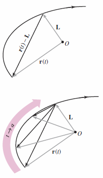If \( \textbf{r} \) is a vector-valued function such that \( \textbf{r}(t) = f(t)\textbf{i}+g(t)\textbf{j}+h(t)\textbf{k} \), then $$ \lim_{t \rightarrow a}\textbf{r}(t) = \left[ \lim_{t \rightarrow a}f(t) \right]\textbf{i} + \left[ \lim_{t \rightarrow a}g(t) \right]\textbf{j} + \left[ \lim_{t \rightarrow a}h(t) \right]\textbf{k} \:\:\:\: \color{red}{ \text{Three Dimensions}} $$ If \( \textbf{r}(t) \) approaches the vector \( \textbf{L} \) as \( t \rightarrow a \), then the vector has the length \( \textbf{r}(t) - \textbf{L}\) approaches 0. Described as an equation \( \| \textbf{r}(t) - \textbf{L} \| \rightarrow 0 \) as \(t \rightarrow a \) as shown in Figure 12.1.6.

Definition 12.1.3 Continuity for a Vector-Valued Function with a Limit

A vector-valued function \( \textbf{r} \) is continuous at the point given by \(t=a\) when the limit for \( \textbf{r}(t) \) exists as \(t \rightarrow a \) and

$$ \lim_{t \rightarrow a} \textbf{r}(t) = \textbf{r}(a).$$

A vector-valued function \( \textbf{r} \) is continuous on an interval \(I\) when it is continuous at every point in the interval. The vector-valued function is continuous at \(t=a\) if and only if each component function is continuous at \(t=a\).

Example 12.1.5 Limit Continuity for a Vector-Valued Function

The vector-valued function in Example 12.1.5 is a parabola for \(a\) values. Figure 12.1.7

Discuss the limit continuity for the vector-valued function $$ \textbf{r}(t) = t \textbf{i} + a\textbf{j} + (a^{2}-t^{2})\textbf{k}$$ at \(t=0\) where \(a\) is a constant. Solution As \(t\) approaches 0, the limit is $$ \lim_{t \rightarrow 0} \textbf{r}(t) $$ $$= \left[ \lim_{t \rightarrow 0} t \right]\textbf{i} + \left[ \lim_{t \rightarrow 0} a \right]\textbf{j} + \left[ \lim_{t \rightarrow 0} (a^{2} -t^{2}) \right]\textbf{k}$$ \(= 0\textbf{i} + a \textbf{j} + a^{2} \textbf{k}\) \(= a \textbf{j} + a^{2} \textbf{k}\) Substituting \(t=0\) into the original equation produces \(\textbf{r}(\color{red}{0}) \) \(= \color{red}{0}\textbf{i} + a \textbf{j} + a^{2} \textbf{k} \) \(= a \textbf{j} + a^{2} \textbf{k} \) 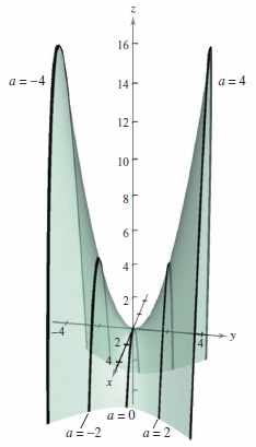which proves that \(\textbf{r} \) is continuous at \(t=0\). By extension the vector-valued function \(\textbf{r} \) is continuous for all real-number values for \(t\). This produces the saddle-shaped curve, shown in Figure 12.1.7. Each value for \(a\) can be viewed as a hyperbolic paraboloid \( y^{2} -x^{2} = z\) intersecting the vertical plane \(y=a\).

Example 12.1.6 Continuity Intervals for a Vector-Valued Function

Determine the interval(s) on which the vector-valued function

\( \textbf{r}(t) = t\textbf{i} + \sqrt{ t+ 1 }\textbf{j} + (t^{2} + 1)\textbf{k} \)

is continuous.
Solution The component functions are \(f(t)=t\), \(g(t)=\sqrt{ t+ 1 }\), and \(h(t)=(t^{2} + 1)\). Both \(f\) and \(h\) are continuous for all real-number values for \(t\). The function \(g\) is continuous only for \( t \geqslant -1\). Therefore \( \textbf{r} \) is continuous on the interval \([-1, \infty )\).

Internal Links

Parent Article: Calculus III 12 Vector-Valued Functions