Calculus III 13.01 Functions with Several Variables

Previous	Calculus III 12 Vector-Valued Functions
Next	Calculus III 13.02 Limits and Continuity

13.01 Functions with Several Variables

• Understand the notation for a function with several variables.
• Sketch the graph for a function with two variables.
• Sketch level curves for a function with two variables.
• Sketch level surfaces for a function with three variables.
• Use software to draw a graph for a function with two variables

Functions with Several Variables

Many familiar functions have two or more variables.

1. The work done by a force, \(W=FD\), has two variables.
2. The volume for a right circular cylinder, \(V=\pi r^{2}h\), has two variables.
3. The volume for a rectangular solid, \(V=lwh\), has three variables.

The notation for a function with two or more variables extends the notation for a function with one variable.

	$$ y = \color{red}{\underbrace{\color{black}{f(x)}}_{\color{red}{\text{1 variable}}}} = x+1 \:\:\:\: \color{red}{ \text{ Function with one variables }}$$
	$$ z = \color{red}{\underbrace{\color{black}{f(x,y)}}_{\color{red}{\text{2 variables}}}} = x^{2}+xy \:\:\:\: \color{red}{ \text{ Function with two variables }}$$
	$$ w = \color{red}{\underbrace{\color{black}{f(x,y,z)}}_{\color{red}{\text{3 variables}}}} = x+2y-3z \:\:\:\: \color{red}{ \text{ Function with three variables }}$$

Definition 13.1.1 A Function with Two Variables

Let \(D\) be real numbers in an ordered pair set. If, to each ordered pair \((x,y)\) in \(D\) there corresponds a unique real number \(f(x,y)\), then \(f\) is a function of \(x\) and \(y\). The set \(D\) is the domain for \(f\), and the corresponding values for \(f(x,y)\) is the range for \(f\). For the function

\(z=f(x,y)\)

\(x\) and \(y\) are called the independent variables and \(z\) is the called the dependent variable.

The definition can be extended to functions with three, four, or \(n\) variables, where the domains are ordered triples \((x_{1},x_{2},x_{3})\), quadruples \((x_{1},x_{2},x_{3},x_{4})\), and \(n\)-tuples \((x_{1},x_{2},...,x_{n})\). In all cases the range is the real number set. The discussion continues with two or three variable functions.

Functions with several variables are often defined as an equation, and unless it is otherwise restricted, the domain is the set for all points for which the equation is defined. For instance, the domain for the function

\( f(x,y)=x^{2}+y^{2} \)

is the entire \(xy\)-plane. Similarly, the domain for

\( f(x,y)=\ln xy \)

is the set for all points \((x,y)\) in the plane for which \(xy>0\). This is all points in the first and third quadrants.

Example 13.1.1 Domains for Functions with Several Variables

Figure 13.1.1

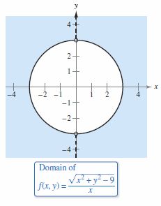
Find the domain for each function. $$\textbf{a. } f(x,y)= \frac{x^{2}+y^{2}-9}{x} $$ $$\textbf{b. } f(x,y,z)= \frac{x}{\sqrt{9-x^{2}-y^{2}-z^{2}}} $$ Solution a. The function \(f\) is defined for all points \((x,y)\) such that \(x \ne 0\) and \(x^{2}+y^{2} \geqslant 9 \). The domain is all points lying on or outside the circle \(x^{2}+y^{2} = 9 \), except those point on the \(y\)-axis, as shown in Figure 13.1.1. b. The function \(g\) is defined for all points \((x,y,z)\) such that \(x^{2}+y^{2}+z^{2} < 9 \). The domain is all points \((x,y,z)\) lying inside a sphere with radius 3 that is centered at the origin.

Functions with several variables can be combined in the same ways as functions with a single variables. The sum, difference, product, and quotient functions with two variables follows.

\((f \pm g)(x,y) \)	\(= f(x,y) \pm g(x,y) \)	Sum or difference
\((fg)(x,y)\)	\(= f(x,y)g(x,y) \)	Product
$$\frac{f}{g} (x,y) $$	$$= \frac{f(x,y)}{g(x,y)}, g(x,y) \ne 0 \:\:\:\: $$	Quotient

Two or more functions with multiple variables have no composite form. However, the composite function \((g \circ h)(x,y)\), where \(g\) is a function with one variable and \(h\) is a function with two variables.

\( (g \circ h)(x,y) = g(h(x,y)) \:\:\:\: \) Composition

The domain for this composite function is all \((x,y)\) in \(h\)'s domain such that \(h(x,y)\) is in \(g\)'s domain. For example, the function

\( f(x,y) = \sqrt{16-4x^{2}-y^{2}} \)

can be viewed as two functions

\( h(x,y) = 16-4x^{2}-y^{2} \)

and

\( g(u) = \sqrt{ u } \).

The domain is all points lying on or inside the ellipse \(4x^{2}+y^{2}=16\).

A polynomial function with two variables is written in the form \(cx^{m}y^{n}\), where \(c\) is a real number and \(m\) and \(n\) are nonnegative integers. For example, the functions

\( f(x,y) = x^{2}+y^{2}+2xy+x+2 \)

and

\( g(x,y) = 3xy^{2}+x-2 \)

are polynomial functions with two variables. A rational function is the quotient with two polynomial functions. Similar terminology is used for functions with more than two variables.

The Graph for a Function with Two Variables

Figure 13.1.2

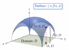
As in life, much can be learned a by rendering an idea as a graphic. The graph for a function \(f\) with two variables is the set for all points \((x, y, z)\) for which \(z = f (x, y )\) and \((x, y)\) is in the \(f\)'s domain. This graph can be interpreted geometrically as a surface in three-dimensions, as discussed in Sections 11.5 and 11.6. In Figure 13.1.2, note that the graph for \(z = f (x, y )\) is a surface whose projection onto the \(xy\)- plane is \(D\), the domain for \( f\). To each point \((x, y)\) in \(D\) there corresponds a point \((x, y,z)\) on the surface, and, conversely, to each point \((x, y,z)\) on the surface there corresponds a point \((x, y)\) in \(D\).

Example 13.1.2 Describing the Graph for a Function with Two Variables

The graph for Example 13.1.2 is an ellipsoid's upper half. Figure 13.1.3

Describe the range for \( f (x, y ) = \sqrt{ 16-4x^{2}-y^{2}} \) and sketch its graph. Solution The domain \(D\) for \(f\) is the point set \((x, y)\) such that \( 16-4x^{2}-y^{2} \geqslant 0 \) Therefore, \(D\) is all points lying on or inside the ellipse described by $$ \frac{x^{2}}{4} + \frac{y^{2}}{16} = 1,$$ on the \(xy\)-plane. The range for \(f\) is all values \(z=f(x,y)\) such that \( 0 \leqslant z \leqslant \sqrt{ 16 } \), or \( 0 \leqslant z \leqslant 4 . 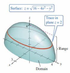\:\:\:\: \) Range for \(f\) A point \((x,y,z)\) is on \(f\)'s graph if and only if \(z\) \(= \sqrt{ 16-4x^{2}-y^{2}} \) \( z^{2} \) \(= 16-4x^{2}-y^{2} \) \( 4x^{2}+y^{2}+z^{2} \) \(= 16 \) $$ \frac{x^{2}}{4} + \frac{y^{2}}{16} +\frac{z^{2}}{16} $$ \(=1, \:\:\:\: 0 \leqslant z \leqslant 4 \) The graph is shown in Figure 13.1.3.

Figure 13.1.4

To sketch a surface in three-dimensions by hand, start by drawing traces in planes parallel to the coordinate planes, as shown in Figure 13.1.3. For example, to find the trace for the surface in the plane \(z=2\), substitute \(z=2\) in the equation \(z = \sqrt{ 16-4x^{2}-y^{2}} \) to produce $$ 2 = \sqrt{ 16-4x^{2}-y^{2}} \rightarrow \frac{x^{2}}{3} + \frac{y^{2}}{12} =1. $$ The trace is an ellipse centered at (0,0,2) with major and minor axes lengths \( 4 \sqrt{3} \text{ and } 2 \sqrt{3}. 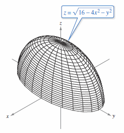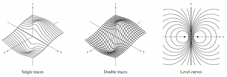\) Traces are also used with three-dimensional graphing utilities. Figure 13.1.4 shows a computer-generated version for the surface given in Example 13.1.2. For this graph, the computer took 25 traces parallel to the \(xy\)-plane and 12 traces in vertical planes. Every three-dimensional graphing utility renders differently so practice with many before choosing one.

Level Curves

A second way to visualize a function with two variables is to use a scalar field in which the scalar

\(z=f(x,y)\)

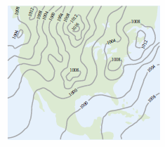
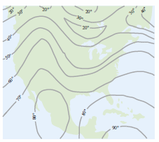
is assigned to the point \((x,y)\). A scalar field can be characterized by level curves (or contour lines) along which the value for \(f(x,y)\) is constant. For instance, the weather map in Figure 13.1.5 shows level curves with equal pressure called isobars. In weather maps for which the level curves represent equal temperature, the level curves are called isotherms, as shown in Figure 13.1.6. Another common use for level curves is in representing electric potential fields called equipotential lines.

Level curves show the lines with equal pressure (isobars), measured in millibars. Figure 13.1.5

Level curves show the lines with equal temperature (isotherms), measured in degrees Fahrenheit. Figure 13.1.6

Figure 13.1.7

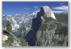
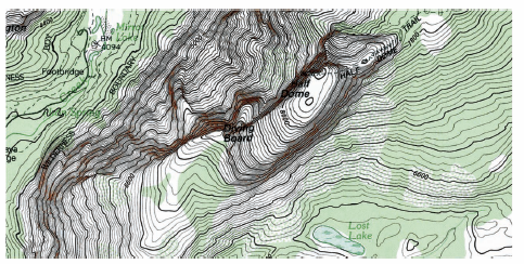
Contour maps are commonly used to show regions on Earth’s surface, with the level curves representing the height above sea level. This map type is called a topographic map. For example, the mountain shown in Figure 13.1.7 is represented by the topographic map in Figure 13.1.8. Figure 13.1.8 A contour map depicts the variation \(z\)'s with respect to \(x\) and \(y\) by the spacing between level curves. More space between level curves indicates that \(z\) is changing slowly, whereas less space indicates a rapid change in \(z\). To produce a good three-dimensional contour map illustration, it is important to choose evenly spaced \(c\)-values.

Example 13.1.3 Sketching a Contour Map for a Hemisphere

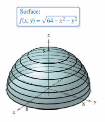
The hemisphere

\( f(x,y) = \sqrt{ 64-x^{2}-y^{2}} \)

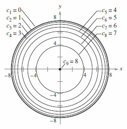
is shown in Figure 13.1.9. Sketch a contour map for this surface using level curves corresponding to \(c=0,1,2,...,8\).
Solution For each value \(c_{n}\), the equation \(f(x,y)=c\) is a circle, or point, in the \(xy\)-plane. For example, when \(c_{1}=0\), the level curve is

\( x^{2}+y^{2} = 64 \:\:\:\: \)Circle with radius 8

which is a circle with radius 8. Figure 13.1.10 shows the nine levels curves for the hemisphere.

Hemisphere Figure 13.1.9

Contour map Figure 13.1.10

Example 13.1.4 Sketching a Contour Map for a Hyperbolic Paraboloid

Hyperbolic paraboloid Figure 13.1.11 Hyperbolic level curves at increments of 2. Figure 13.1.12

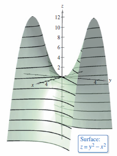
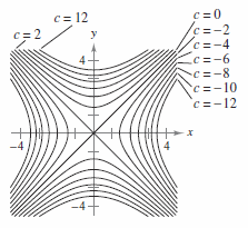
The hyperbolic paraboloid \(z=y^{2}-x^{2}\) is shown in Figure 13.1.11. Sketch a contour map for this surface. Solution For each value \(c_{n}\), let \(f(x,y)=c\) and sketch the resulting level curve in the \(xy\)-plane. For this function, each level curve in the \(xy\)-plane. For this function, each level curve where \(c \ne 0 \) is a hyperbola with asymptotes at lines \(y= \pm x\). When \(c < 0\), the transverse axis is horizontal. For instance, the level curve for \(c=-4\) is $$ \frac{x^{2}}{2^{2}} - \frac{y^{2}}{2^{2}} = 1. $$ When \(c > 0\), the transverse axis is vertical. For instance, the level curve for \(c=4\) is $$ \frac{y^{2}}{2^{2}} - \frac{x^{2}}{2^{2}} = 1. $$ When \( c = 0\), the level curve is the degenerate conic representing the intersecting asymptotes, as shown in Figure 13.1.12.

Example 13.1.5 The Cobb-Douglas Production Function

Level curves at increments of 10,000. Figure 13.1.13

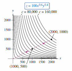
The Cobb-Douglas production function is a function with two variables used in economics. It is used as a model to represent the units produced by varying labor and capital. If \(x\) measures the labor units and \(y\) measures the capital units, then the units produced is $$ f(x,y)= Cx^{a}y^{1-a}$$ where \(C\) and \(a\) are constants with \(0< a < 1.\) A toy manufacturer estimates a production function to be $$ f(x,y)= 100x^{0.6}y^{0.4}$$ where \(x\) is the labor units and \(y\) is the capital units. Compare the production level where \(x=1000\) and \(y=500\) with the production level when \(x=2000\) and \(y=1000\). Solution When \(x=1000\) and \(y=500\), the production level is \( f( \color{red}{1000}, \color{red}{500})=100( \color{red}{1000}^{0.6})(\color{red}{500}^{0.4}) \approx 75,786. \) When \(x=2000\) and \(y=1000\), the production level is \( f( \color{red}{2000}, \color{red}{1000})=100( \color{red}{2000}^{0.6})(\color{red}{1000}^{0.4}) \approx 151,572. \) The level curves for \(z=f(x,y)\) are shown in Figure 13.1.13. Note that by doubling both \(x\) and \(y\), the production level is doubled as well.

Level Surfaces

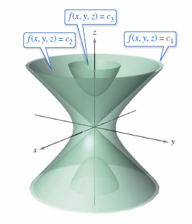
The level curve can be extended by one dimension to define a level surface. If \(f\) is a function with three variables and \(c\) is a constant, then the graph for the equation

\( f(x,y,z)=c\)

is a level surface for the function \(f\), as shown in Figure 13.1.14.

Level surface for \(f\)
Figure 13.1.14

Example 13.1.6 Level Surfaces in Three Dimensions

Figure 13.1.15

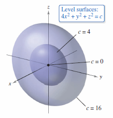
Describe the level surfaces for \( f(x,y,z) = 4x^{2}+y^{2}+z^{2}.\) Solution Each level surface has an equation with the form \( 4x^{2}+y^{2}+z^{2} = c . \:\:\:\: \)Equation for level surface The level surfaces are ellipsoids with circular cross sections parallel to the \(yz\)-plane. As \(c\) increases, the radii for the circular cross sections increase according to \(c\)'s square root. For example, the level surfaces corresponding to the values \(c = 0\), \(c = 4\), and \(c = 16\) are as follows. \( 4x^{2}+y^{2}+z^{2} \) \(= 0 \) Level surface for \(c=0\) (single point) $$ \frac{x^{2}}{1} + \frac{y^{2}}{4} + \frac{z^{2}}{4} $$ \(=1 \) Level surface for \(c=4\) (ellipsoid) $$ \frac{x^{2}}{4} + \frac{y^{2}}{16} + \frac{z^{2}}{16} $$ \(= 1\) Level surface for \(c=16\) (ellipsoid) The level surfaces are shown in Figure 13.1.15. If the function represented the temperature at the point \((x,y,z)\), then the level surfaces would be called isothermal surfaces.

Computer Graphics

Figure 13.1.16

Most three-dimensional graphing programs use a trace analysis to render a three-dimensional image on a two-dimensional media. The program requires at least the equation for the surface in the \(xy\)-plane and possibly the trace count. For instance, to render the surface \( f(x,y)=(x^{2}+y^{2}) e^{1-x^{2}-y^{2}} \) you might choose the following bounds for \(x\), \(y\), and \(z\). 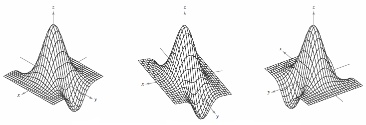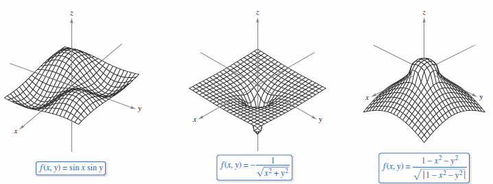\( -3 \leqslant x \leqslant 3 \)     Bounds for \(x\) \( -3 \leqslant y \leqslant 3 \)     Bounds for \(y\) \(\hphantom{-} 0 \leqslant z \leqslant 3 \)     Bounds for \(z\) Figure 13.1.16 shows a computer-generated graph for this surface using 26 traces taken parallel to the \(yz\)-plane. To enhance the three-dimensional effect, the program uses a “hidden line” routine. It begins by plotting the traces in the foreground, those corresponding to the largest \(x\)-values, and then, as each new trace is plotted, the program determines whether all or only part of the next trace should be shown. The graphs in Figures 13.1.17, 13.1.18, and 13.1.19 show different surfaces that were plotted by computer. Always remember to rotate the graph until you see an optimal view.

The graph for \(f(x,y)=(2-y^{2}+x^{2})e^{1-x^{2}-(y^{2}/4)}\)
Figure 13.1.17

The graph for
$$ f(x,y)= \frac{-4x}{x^{2}+y^{2}+1} $$
Figure 13.1.18

Figure 13.1.19

Internal Links

Parent Article: Calculus III 13 Functions with Several Variables