Calculus III 13.09 Extrema Applications
| Previous | Calculus III 13.08 Extrema for Functions with Two Variables |
| Next | Calculus III 13.10 Lagrange Multipliers |
13.9 Extrema Applications
- Solve optimization problems involving functions with multiple.
- Least squares method.
Applied Optimization Problems
Example 13.9.1 Finding Maximum Volume
|
|
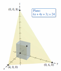
A rectangular box is resting on the \(xy\)-plane with one vertex at the origin. The opposite vertex lies in the plane
as shown in Figure 13.9.1. Find the box's maximum volume.
Find the partial derivatives for \(V\).
Note that the first partial derivatives are defined for all \(x\) and \(y\). By setting \(V_{x}(x,y) \) and \(V_{y}(x,y) \) equal to zero and solving the critical points \((0,0)\), \((4/3,2)\) are produced. At \((0,0)\), the volume is zero, a global minimum. At \((4/3,2)\) the Second Partials Test can be applied.
Because
and
the maximum volume is
Note that the volume is zero at the boundary points for the triangular domain for \(V\). |
Example 13.9.2 Finding the Maximum Profit
Extrema applications in economics and business often involve more than one independent variable. For instance, a company may produce a product in several models. The price per unit and profit per unit are usually different for each model. The demand for each model is often a function with the prices for the other models, as well as its own price, are variables.
An electronics manufacturer determines that the profit \(P\), in dollars, obtained by producing and selling LCD televisions, \(x\) units, and plasma televisions, \(y\) units, is approximated by the model
- \(P(x,y) = 8x+10y-(0.001)(x^{2}+xy+y^{2}) - 10,000. \)
Find the production level that produces a maximum profit. What is the maximum profit?
Solution The partial derivatives for the profit function are
- \( P_{x}(x,y) = 8-(0.001)(2x+y) \)
and
- \(P_{y}(x,y) = 10-(0.001)(x+2y). \)
Setting these partial derivatives equal to zero produces the linear equations,
| \( 8-(0.001)(2x+y) \) | \(= 0 \) | \( \rightarrow \) | \( 2x+y \) | \(=8000 \) | \( \rightarrow \) | \(x=2000\) |
| \( 10-(0.001)(x+2y) \) | \(= 0\) | \( \rightarrow \) | \(x+2y \) | \( 10,000 \) | \( \rightarrow \) | \(y=4000. \) |
The second partial derivatives for \(P\) are
| \(P_{xx}(2000,4000) \) | \(= -0.002 \) |
| \(P_{yy}(2000,4000) \) | \(= -0.002 \) |
| \(P_{xy}(2000,4000) \) | \(= -0.001. \) |
Because \(P_{xx} < 0 \) and
- \( P_{xx}(2000,4000) P_{yy}(2000,4000) - [P_{xy}(2000,4000)]^{2} = (-0.002)^{2}-(-0.001)^{2}\)
is greater than zero. The conclusion is that a production level with \(x=2000\) units and \(y=4000\) units yields a maximum profit. The maximum profit is
- \(P(2000,4000) = $18,000.\)
Least Squares Method
Many examples have use mathematical models. Example 13.9.2 involves a quadratic model for profit. There are several ways to develop such models; this one is called the Least Squares Method.
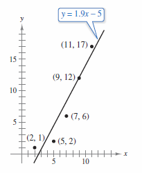
In constructing a model to represent a particular phenomenon, the goals are simplicity and accuracy, which sometimes conflict. For instance, a simple linear model for the points in Figure 13.9.2 is
- \( y=1.9x - 5\)
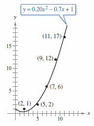
Figure 13.9.3 shows that by choosing the slightly more complicated quadratic model
- \( y=0.20x^{2} -0.7x+1\)
greater accuracy is achieved.
|
|
|
As a measure for how well the model \(y=f(x)\) fits the point collection
- \( \{(x_{1},y_{1}),(x_{2},y_{2}),(x_{3},y_{3}),...,(x_{n},y_{n})\}, \)
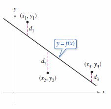
take the differences between the actual \(y\)-values and the values given by the model, square them, sum them, to produce the sum of the squared errors.
- $$ S = \sum_{i=1}^{n} [f(x_{i})-y_{i}]^{2} \:\:\:\: \color{red}{ \text{ Sum of the squared errors.}}$$
|
|
Graphically, \(S\) can be interpreted as the sum of the squares of the vertical distances between \(f\)'s graph and the given points in the plane, as shown in Figure 13.9.4. If the model is perfect, then \(S = 0\). A less than perfect model minimizes \(S\). For instance, the sum of the squared errors for the linear model in Figure 13.9.2 is
Statisticians call the linear model that minimizes \(S\) the least squares regression line. The proof that this line actually minimizes \(S\) involves the minimizing a function with two variables. |
Theorem 13.9.1 Least Squares Regression Line
The least squares regression line for \( \{(x_{1},y_{1}),(x_{2},y_{2}),(x_{3},y_{3}),...,(x_{n},y_{n})\} \) is given by \(f(x)=ax+ b\), where
| \( a= \) | $$ n \sum_{i=1}^{n} x_{i}y_{i} - \sum_{i=1}^{n} x_{i}\sum_{i=1}^{n}y_{i} $$ |
| | |
| $$ n \sum_{i=1}^{n} x_{i}^{2} - \left( \sum_{i=1}^{n} x_{i} \right)^{2}$$ |
and
- $$ b=\frac{1}{n} \left( \sum_{i=1}^{n} y_{i} - a \sum_{i=1}^{n} x_{i} \right). $$
Proof Let \(S(a,b)\) represent the sum of the squared errors for the model
- \(f(x)=ax+b\)
and the given point set. That is
| \(S(a,b)\) | $$= \sum_{i=1}^{n} [f(x_{i}) - y_{i}]^{2} $$ |
| $$= \sum_{i=1}^{n} (ax_{i} +b - y_{i})^{2}$$ |
where the points \((x_{i},y_{i})\) represents constants. Because \(S\) is a function for \(a\) and \(b\), the methods in Section 13.8 to find the minimum value for \(S\). The first partial derivatives are
| \(S_{a}(a,b)\) | $$= \sum_{i=1}^{n} 2x_{i}(ax_{i} +b - y_{i})$$ |
| $$= 2a\sum_{i=1}^{n} x_{i}^{2} + 2b \sum_{i=1}^{n} x_{i} - 2 \sum_{i=1}^{n} x_{i}y_{i} $$ |
and
| \(S_{b}(a,b)\) | $$= \sum_{i=1}^{n} 2(ax_{i} +b - y_{i})$$ |
| $$= 2a\sum_{i=1}^{n} x_{i}^{2} + 2nb - 2 \sum_{i=1}^{n} y_{i}. $$ |
Set both partial derivatives equal to zero and solve for \(a\) and \(b\).
Example 13.9.3 Finding the Least Squares Regression Line
|
|
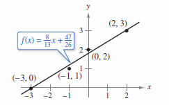
Find the least squares regression line for the points
Solution The Table 13.9.1 shows the calculations involved in finding the least squares regression line using \(n=4\).
Applying Theorem 13.9.1 produces
and
The least squares regression line is
as shown in Figure 13.9.5.
| ||||||||||||||||||||||||||||||||||||||||||
Internal Links
Parent Article: Calculus III 13 Functions with Several Variables
