Calculus II 06.01 Slope Fields and Euler's Method
| Previous | Calculus I |
| Next | Calculus II 06.02 Differential Equations Growth and Decay |
Contents
6.1 Slope Fields and Euler's Method
- Solve differential equations using initial conditions.
- Approximate solutions for differential equations using slope fields.
- Use Euler’s Method to approximate solutions for differential equations.
General and Particular Solutions
Physical phenomena can be described by differential equations. A differential equation in \(x\) and \(y\) is an equation that involves \(x\), \(y\), and \(y\)'s derivatives. For example,
- \(2xy^{\prime}-3y=0\:\:\:\:\) Differential equation
is a differential equation. Phenomena involving radioactive decay, population growth, and Newton's Law of Cooling can be expressed as differential equations.
A function \(y=f(x)\) is called a solution for a differential equation if the equation is satisfied when \(y\) and its derivatives are replaced by \(f(x)\) and its derivatives. For example, differentiation and substitution would show that \(y=e^{-2x}\) is a solution for the differential equation \(y^{\prime}+2y=0\). Every solution for this differential equation has the form
- \(y=Ce^{-2x}\:\:\:\:\) General solution for \(y^{\prime}+2y=0\)
where \(C\) is any real number. This solution is called the general solution. Differential equations with singular solutions, that cannot be written as specials cases for the general solution, are not covered in this discussion.
The differential equation's order is determined by the highest-order derivative in the equation. For instance, \(y^{\prime}=4y\) is a first-order differential equation. First-order linear differential equations are discussed in Section 6.4. In Section 4.1, Example 4.1.9, the second-order differential equation \( s^{\prime \prime}(t)=-32\) has the general solution
- \(s(t)=-16t^{2}+C_{1}t+C_{2}\:\:\:\:\) General solution for \( s^{\prime \prime}(t)=-32 \)
which contains two arbitrary constants. A differential equation with order \(n\) has a general solution with \(n\) arbitrary constants.
Example 6.1.1 Verifying Solutions
Determine whether the funtion is a solution for the differential equation \( y^{\prime \prime}-y=0 \).
- a. \(y=\sin x\)
- b. \(y=4e^{-x}\)
- c. \(y=Ce^{x}\)
Solution
a. Because \(y=4e^{-x}\), \(y^{\prime}=\cos x\), and \(y^{\prime \prime}=-\sin x\), if follows that
- \(y^{\prime \prime}-y=-\sin x\), \(-\sin x=-2\sin\), \(x \neq 0\).
Therefore \(y=\sin x\) is not a solution. b. Because \(y=4e^{-x}\), \(y^{\prime}=-4e^{-x}\), and \(y^{\prime \prime}=4e^{-x}\), it follows that
- \(y^{\prime \prime}-y=4e^{-x}-4e^{-x}=0\).
Therefore \(y=4e^{-x}\) is a solution.
c. Because \(y=Ce^{x}\), \(y^{\prime}=Ce^{x}\), and \(y^{\prime \prime}=Ce^{x}\), it follows that
- \(y^{\prime \prime}-y=Ce^{x}-Ce^{x}=0\).
Therefore \(y=Ce^{x}\) is a solution for any \(C\) value.
|
|
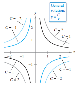
The general solution for a first-order differential equation produces a curve family known as solution curves, with one curve for each value assigned to the arbitrary constant. For example, you can verify that every function with the from
is a solution for the differential equation
Figure 6.1.1 shows four curves corresponding to different values for \(C\). As discussed in Section 4.1, particular solutions for a differential equation are obtained from initial conditions that give provide specific values for the dependent variable or its derivative and for the independent variable. The term “initial condition” stems from the fact that, often in problems involving time, the value for the dependent variable or a derivative is known at the initial time \(t=0\). For instance, the second-order differential equation
having the solution
might have the following conditions.
These initial conditions yield the particular solution
|
Example 6.1.2 Finding a Particular Solution
For the differential equation
- \(xy^{\prime}-3y=0\)
verify that \(y=Cx^{3}\) is a solution. Then find the particular solution determined by the initial condition \(y=2\) when \(x=-3\). To determine a particular solution, each initial condition must map to a constant in the general solution.
Solution You know that \(y=Cx^{3}\) is a solution because \(y^{\prime}=3Cx^{2}\) and
- \(xy^{\prime}-3y=x(3Cx^{2})-3(Cx^{3})-0\).
Furthermore, the initial condition \(y=2\) when \(x= -3\) yields
| \(y=Cx^{3}\) | General solution |
| \(2=C(-3)^{3}\) | Substitute initial condition. |
| \(-\frac{2}{27}=C\) | Solve for \(C\) |
| and you can conclude that the particular solution is</span> | |
| \(y=\frac{2x^{3}}{27}\). | Particular solution |
Try checking this solution by substituting for and in the original differential equation.
Slope Fields
Solving a differential equation analytically can be difficult or even impossible. However, there is a graphical approach you can use to learn a lot about the solution. Consider the differential equation
- \(y^{\prime}=F(x,y)\:\:\:\: \) Differential equation
where \(F(x,y)\) is some expression in \(x\) and \(y\). At each point in the \(xy\)-plane where \(F\) is defined, the differential equation determines the solution's slope \(F(x,y)\) at that point. Draw short line segments with slope \(F(x,y)\) at selected points \((x,y)\) in the domain forms a slope field[1], or a direction field, for the differential equation \(y^{\prime}=F(x,y)\). Each line segment has the same slope as the solution curve through that point. Plotting the slope field over a solution space produces a graphic that describes all the solution trends for that space. See Example 6.1.4 below.
Example 6.1.3 Sketching a Slope Field
|
|
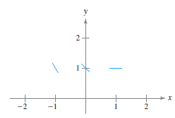
Sketch a slope field for the differential equation \(y^{\prime}=x-y\) for the points (-1,1), (0,1), and (1,1).
The slope at each point can be found as shown.
Draw short line segments at the three points with their respective slopes, as shown in Figure 6.1.2. |
Example 6.1.4 Identifying Slope Fields for Differential Equations
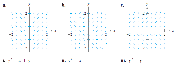
Match each slope field with its differential equation.
Solution
- a. You can see that the slope at any point along the \(x\)-axis is 0. The only equation that satisfies this condition is \(y^{\prime}=x\). So, the graph matches equation (ii).
- b. You can see that the slope at the point (1,-1) is 0. The only equation that satisfies this condition is \(y^{\prime}=x+y\). So, the graph matches equation (i).
- c. You can see that the slope at any point along the \(x\)-axis is 0. The only equation that satisfies this condition is \(y^{\prime}=y\). So, the graph matches equation (iii).
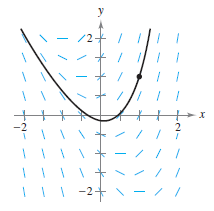
A solution curve for the differential equation \(y^{\prime \prime}=F(x,y)\) is simply a curve in the \(xy\)-plane whose tangent line at each point \((x,y)\) has slope equal to \(F(x,y)\). This is illustrated in Example 6.1.5.
Example 6.1.5 Sketching a Solution Using a Slope Field
Sketch a slope field for the differential equation
- \(y^{\prime}=2x+y\).
Use the slope field to sketch the solution that passes through the point (1,1).
Solution Make a table showing the slopes at several points. The table shown is a
small sample. The slopes at many other points should be calculated to get a representative
slope field.
| Table 6.1.1 | ||||||||||
|---|---|---|---|---|---|---|---|---|---|---|
| \(x\) | -2 | -2 | -1 | -1 | 0 | 0 | 1 | 1 | 2 | 2 |
| \(y\) | -1 | 1 | -1 | 1 | -1 | 1 | -1 | 1 | -1 | 1 |
| \(y^{\prime}=2x+y\) | -5 | -3 | -3 | -1 | -1 | 1 | 1 | 3 | 3 | 5 |
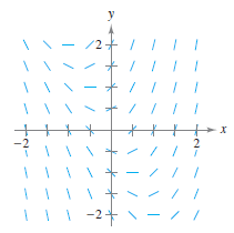
Next, draw line segments at the points with their respective slopes, as shown in Figure 6.1.3.
After the slope field is drawn, start at the initial point (1,1) and move to the right in the direction of the line segment. Continue to draw the solution curve so that it moves parallel to the nearby line segments. Do the same to (1,1)'s left. The resulting solution is shown in Figure 6.1.5. In Example 6.1.5, note that the slope field shows that increases to infinity as increases. Note that the slope filed show that \(y^{\prime}\) increase to infinity as \(x\) increases.
Euler's Method
|
|
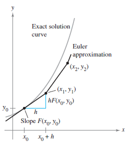
Euler's Method is a numerical approach to approximating the solution for
that passes through the point \((x_{0},y_{0})\). The solution's graph passes through the point \((x_{0},y_{0})\) and has the slope \(F(x_{0},y_{0})\) at that point. This produces a "starting point" for approximating the solution. Connect straight lines in a series along the curve. Using a small constant \(h\), at each step, move along the tangent line until arriving at the point \(F(x_{1},y_{1})\), where
as shown in Figure 6.1.6. Using \((x_{1},y_{1})\) as the new starting point, repeat the process to obtain the next point \((x_{2},y_{2})\). Continue along the slope for \(n\) steps. The smaller \(h\) is, the greater the accuracy. The variables \(x_{i}\) and \(y_{i}\) progress from \(0\) to \(n\) as shown below
|
Example 6.1.6 Approximating a Solution using Euler's Method
|
|
Use Euler's Method to approximate the exact solution to the differential equation
passing through the point (0,1). Use a step where \(h= 0.1\).
and the first three approximations are
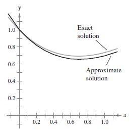
The first ten approximations are shown in the table below. Plotting the approximate solutions produces a graph as shown in Figure 6.1.7.
Figure 6.1.7 compares this exact solution with the approximate solution obtained in Example 6.1.6. | |||||||||||||||||||||||||||||||||||||||||||||||||||
Internal Links
Parent Article: Calculus II 06 Differential Equations
