Calculus II 06.02 Differential Equations Growth and Decay

Previous	Calculus II 06.01 Slope Fields and Euler's Method
Next	Calculus II 06.03 Separating Variables and the Logistic Equation

6.2 Differential Equations: Growth and Decay

• Solve a simple differential equation by separation of variables.
• Model growth and decay in applied problems using exponential functions.

Differential Equations

Euler’s Method, Section 6.1, uses slope fields to approximate solutions for first order forms \(y^{\prime}=f(x)\) and second order forms \(y^{\prime \prime}=f(x)\) differential equations. This section discusses using separation of variables to solve more general differential equations by putting the equal sign between the variables. as described in Example 6.2.1. Section 6.3 discusses this strategy in greater depth.

Example 6.2.1 Solving a Differential Equation

\(y^{\prime}=\frac{2x}{y}\)	Original Equation
\(yy^{\prime}=2x\)	Multiply both sides by \(y\)
\(\int yy^{\prime}\:dx=\int 2x\:dx\)	Integrate with respect to \(x\)
\(\int y\:dy=\int 2x\:dx\)	\(dy=y^{\prime}\:dx\)
\(\frac{1}{2}y^{2}=x^{2}+C_{1}\)	Apply Power Rule
\(y^{2}-2x^{2}=C\)	Rewrite letting \(C=2C_{1}\)
\(y^{2}-2x^{2}=C\)	The general solution

When integrating both sides as in Example 6.2.1, there is no need to add a constant to both sides because the constants \(C_{2}\) and \(C_{3}\) cancel each other out.

\(\int y\:dy=\int 2x\:dx\)

\(\frac{1}{2}y^{2}+C_{2}=x^{2}+C_{3}\)

\(\frac{1}{2}y^{2}=x^{2}+(C_{3}-C_{2})\)

\(\frac{1}{2}y^{2}=x^{2}+C_{1}\)

Some people prefer the Leibniz Notation[1] and differentials when separating variables. The solution to Example 6.2.1 is shown below using this notation.

\(\frac{dy}{dx}=\frac{2x}{y}\:dx\)

\(y\:dy=2x\:dx\)

\(\int y\:dy=\int 2x\:dx\)

\(\frac{1}{2}y^{2}=x^{2}+C_{1}\)

\(y^{2}-2x^{2}=C\)

Growth and Decay Models

A variable's change rate is proportional to the value for \(y\). When \(y\) is a function of time \(t\), the proportion can be written as shown in Figure 6.2.1.

Figure 6.2.1

The general solution for this differential equation is given in Theorem 6.2.1.

Theorem 6.2.1 Exponential Growth and Decay Model

If \(y\) is a differential function for \(t\) such that \(y>0\) and \(y^{\prime}=ky\) for some constant \(k\), then

\(y=Ce^{kt}\)

where \(C\) is the initial value for \(y\), and \(k\) is the proportionality constant. Exponential growth occurs when \(k>0\), and exponential decay occurs when \(k<0\).
Proof

\(y^{\prime}=ky\)	Original Equation
\(\frac{y^{\prime}}{y}=k\)	Separate Variables
\(\int \frac{y^{\prime}}{y}\:dt=\int k\:dt \:\:\:\: \)	Integrate with respect to \(t\)
\(\int \frac{1}{y}\:dy=\int k\:dt \:\:\:\: \)	\(dy=y^{\prime}\:dt\)
\(\ln y=kt+C_{1}\)	Find antiderivatives for both sides
\(y=e^{kt}e^{C_{1}}\)	Solve for \(y\)
\(y=Ce^{kt}\)	Let \(C=e^{C_{1}}\)

All solutions for \(y^{\prime}=ky\) have the form \(y=Ce^{kt}\). Remember that you can differentiate the function \(y=Ce^{kt}\) with respect to \(t\) to verify that \(y^{\prime}=ky\).

Example 6.2.2 Using an Exponential Growth Model

Figure 6.2.2 If the change rate for \(y\) is proportional to \(y\), then \(y\) follows an exponential model.

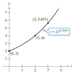
The change rate for \(y\) is proportional to \(y\) as \(t\) changes. When \(t=0\), \(y=2\) and when \(t=2\), \(y=4\). What is \(y\) when \(t=3\)? Solution Because \(y^{\prime}=ky\), you know that \(y\) and \(t\) are related by the equation \(y=Ce^{kt}\). You can find the values for the constants \(C\) and \(k\) and by applying the initial conditions as described below. \(2=Ce^{0}\rightarrow C=2\) When \(t=0\), \(y=2\) \(4=2e^{2k}\rightarrow k=\frac{1}{2}\ln 2 \approx 0.3466 \:\:\:\: \) When t=2, y=4 The model is \(y=2e^{0.3466t}\). When \(t=3\), \(y\) is \(2e^{0.3466({\color{Red} 3})} \approx 5.657\) as in Figure 6.2.2. Using logarithmic properties \(k\) can also be written as \(\ln\sqrt{2}\). This changes the model to \(y=2e^{(\ln\sqrt{2})t}\), which can be rewritten as \(y=2(\sqrt{2})^{t}\).

Radioactive Decay

Radioactive decay is measured as half-life[2] — the years required for half the atoms in a sample to decay. The decay rate is proportional to the amount present. The more material, the higher the rate. The less material, the lower the rate. The half-lives for some common radioactive isotopes are listed below.

Uranium \(^{238}U\)	4,470,000,000 years
Plutonium \(^{238}Pu\)	24,100 years
Carbon \(^{14}C\)	5715 years
Radium \(^{226}Ra\)	1599 years
Einsteinium \(^{254}Es \:\:\:\: \)	276 days
Radon \(^{222}Rn\)	3.82 days
Nobelium \(^{257}No\)	25 seconds

Example 6.2.3 Radioactive Decay

Ten grams of the plutonium isotope \({}^{239}Pu\) were released in a nuclear accident. How long will it take for the 10 grams to decay to 1 gram?
Solution Let \(y\) represent the plutonium's mass (in grams). Because the decay rate is proportional to \(y\), yields

\(y=Ce^{kt}\)

where \(t\) is the time in years. To find the values for \(C\) and \(k\), apply the initial conditions. Using the fact that \(y=10\) when \(t=0\) the general solution can be written as

\(10=Ce^{k(0)}\rightarrow 10=Ce^{0}\)

which implies that \(C=10\). The half-life for \({}^{239}Pu\) is 24,100 years, which yields \(y= 10/2 = 5\) when \(t=24,100\), which produces

\(5=10e^{k(24,100)}\))
\(\frac {1}{2}=e^{24,100k}\)
\(\frac {1}{24,100}\ln \frac {1}{2}=k\)
\(-0.000028761 \approx k\)
The model is
\(y=10e^{-0.000028761t} \:\:\:\: \)	Half-life model

Solve for \(t\) to find long it takes for 10 grams to decay to 1 gram

\(1=10e^{-0.000028761t}\)

The solution is approximately 80,059 years.
Notice that in an exponential growth or decay problem, it is easy to solve for \(C\) when the value for \(y\) at \(t=0\) is known. Example 6.2.4 demonstrates a procedure for solving for \(C\) and \(k\) when \(y\) at \(t=0\) is not known.

Example 6.2.4 Population Growth

Figure 6.2.3

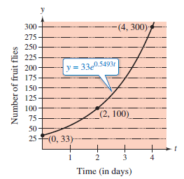
An experimental fruit fly population increases according to the Law of Exponential Growth[3]. On the second day there were 100 flies. After the fourth day there were 300 flies. Approximately how many flies were in the original population? Solution Let \(y=Ce^{kt}\) be the fly count at time \(t\), where \(t\) is measured in days. Note that \(y\) is continuous, whereas the fly count is discrete. Because \(y=100\) when \(t=2\) and \(y=300\) when \(t=4\) yields \(100=Ce^{2k}\) and \(300=Ce^{4k}\) Set them equal and solve to find the growth model. \(C\) \(= 100e^{-2k}\) Solve for \(C\) \(300\) \(= 100e^{-2k}e^{4k}\) Substitute back in \(300\) \(= 100e^{2k}\) \(3\) \(= e^{2k}\) \(\ln 3\) \(= 2k\) \( 1/2 \ln 3\) \(= k\) \( 0.5493\) \(\approx k\) Plugging this back into the general solution produces the growth model \(y=Ce^{0.5493t}\) To solve for \(C\) substitute \(y=100\) when \(t=2\) to produce \(100\) \(=Ce^{0.5493(2)} \) \(C\) \(=100e^{-1.0986} \approx 33\) The original population, when \(t=0\), was \(y=C=33\) flies, as shown in Figure 6.2.3. Fractional flies are not allowed.

Example 6.2.5 Declining Sales

Figure 6.2.4

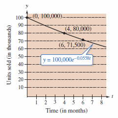
Four months after it stops advertising, a manufacturing company notices that its sales have dropped from 100,000 units per month to 80,000 units per month. The sales decline at exponential pattern rate. What will the sales be after another 2 months? Solution Let \(y=Ce^{kt}\) be the exponential decay model, where \(t\) is measured in months. At the initial condition, \(t=0\), \(C=100,000\). Take the initial conditions, \(y=80,000\) when \(t=4\), and solve for \(k\) \(80,000\) \(=100,00e^{4k} \) \(0.8\) \(= e^{4k}\) \(\ln (0.8)\) \(= 4k \) \( -0.05588 \) \(\approx k \) After another 2 months, \(t=6\), the monthly sales rate will be \(y=100,000e^{-0.05588(6)} \approx 71,500\) units, as shown in Figure 6.2.4.

Example 6.2.6 Newton’s Law of Cooling[4]

Figure 6.2.5

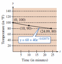
Newton’s Law of Cooling states that the change rate in the temperature for an object is proportional to the difference between the object’s temperature and the surrounding medium's temperature. Let \(y\) represent the temperature in °F for an object in a room whose temperature is kept at a constant 60°. The object cools from 100° to 90° in 10 minutes. How much longer will it take for the object's temperature to decrease to 80°? Solution From Newton’s Law of Cooling, you know that the rate of change in is proportional to the difference between and 60. This can be written as \(y^{\prime}=k(y-60), 80 \leqslant y \leqslant 100\) To solve this differential equation separate the variables, as shown. $$ \frac{dy}{dt} $$ $$=k(y-60) $$ Differential Equation $$ \left ( \frac{1}{y-60} \right ) dy$$ $$ =k\:dt \:\:\:\: $$ Separate the variables $$ \int \frac {1}{y-60}dy$$ $$=\int k\:dt $$ Integrate each side \(\ln | y-60 | \) \(=kt+C_{1}\) Find antiderivative for both sides Now solve for \(k\). \(y-60\) \(=e^{kt+C_{1}} \) \(y\) \(= 60+Ce^{kt}\) \(C=e^{C_{1}}\) \(100\) \(=60+Ce^{k(0)} \) Use \(y=100\) when \(t=0\) \(100\) \(=60+C\) Indicates \(C=40\) when \(y=90\) and \(t=10\) \(90\) \(=60+40e^{k(10)}\) \(30\) \(=40e^{10k}\) \(1/10 \ln 3/4 \) \(=k\) \(-0.02877\) \( \approx k\) \(y=60+40e^{-0.02877t} \) The Cooling Model Plugging in \(y=80\) produces \(80\) \(= 60+40e^{-0.02877t}\) \(20\) \(=40e^{-0.02877t} \) \(\frac{1}{2} \) \(=e^{-0.02877t} \) \(\ln \frac{1}{2} \) \(= -0.02877t\) \(t\) \(\approx 24.09\) minutes It will require about 14.09 more minutes for the object to cool to to 80°, as shown in Figure 6.2.5.

Internal Links

Parent Article: Calculus II 06 Differential Equations