Algorithm Design and Analysis
Algorithms Design and Analysis
Contents
Topics Covered
Correctness, Time And Space Complexity, Insertion-Sort, Growth Of Functions, Asymptotic Notation, Big-Oh, Big-Omega, Big-Theta, Upper Bound, Lower Bound, Tight Bounds, Divide-And-Conquer, Merge-Sort, Recurrences, Substitution Method, Recursion-Tree Method, Master Theorem, Divide And Conquer.
Problems
Main Article: Algorithm Design and Analysis (Problems)
Exercises and Problems for "Algorithm Design and Analysis".
Algorithm
What is an algorithm?[1]
An informal definition is:
An algorithm is any well-defined computational procedure that takes some value, or set of values, as input and produces some value, or set of values, as output. An algorithm is thus a sequence of computational steps that transform the input into the output.
- An instance of a problem is the input, that satisfies the problem statement, needed to compute a solution to the problem.
- Correctness. An algorithm is correct if, for every instance, it halts with the correct output.
- Incorrect. An incorrect algorithm will halt with an invalid output, or never halt, or halt undecidable output.
- Solves. A correct algorithm halts with the correct output.
Merge-Sort vs. Insertion Sort
$$n^{2}=n \cdot lg( n ) $$
$$n \cdot n = n \cdot lg ( n ) $$
$$n = lg ( n )$$
Traveling Salesman, NP-Complete
Algorithm as a Technology.
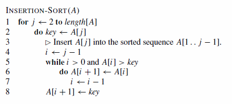
- Insertion Sort
Keys are sorted in the input array by swapping key pairs where \(key_{1} > key_{2}\).
Loop Invariant[2] Is true before and after each iteration. But no necessarily during each iteration. The loop invariant has three properties.
- Initialization: It is true prior to the loop's first iteration.
- Maintenance: If it is true before a loop iteration, it remains true before the next iteration.
- Termination: When the loop terminates, the invariant gives us a useful property that helps show that the algorithm is correct.
Analyzing Algorithms
Predicting the resources the algorithm requires. These include time, cycles, pipelines, RAM, storage, electricity, money, and opportunity costs.
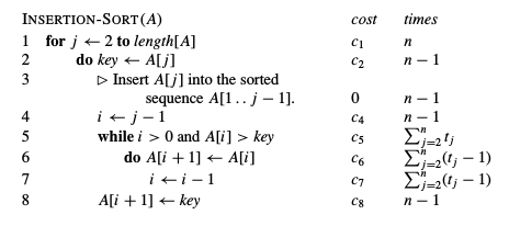
The algorithm's run time sums the time for each statement executed. A statement that takes \(c_{i}\) steps to execute and is executed \(n\) times will contribute \(c_{i}n\) to the total running time. To compute \(T(n)\), the running time for Insertion-Sort, sum the products for cost and time columns in Figure 2, producing $$T(n) = c_{i}n + c_{2}(n-1)+ c_{4}(n-1)+c_{5} \sum^{n}_{j=2} t_{j} + c_{6}\sum^{n}_{j=2} (t_{j}-1) +c_{7}\sum^{n}_{j=2} (t_{j}-1)+c_{8}(n-1).$$
Cases for an algorithm come in three types:
- Best Case - Shortest time for an unsorted input, lower bounds
- Average Case - Time for most inputs, average bounds
- Worse Case - Longest time for an unsorted input, upper bounds
Order of Growth
How does the cost and run time increase as the input increases in size and complexity?
Designing Algorithms
Insertion-Sort is incremental, now for divide-and-conquer. An algorithm that recursively calls itself as it divides the input into smaller and smaller bit-sized chunks follows a divide-and-conquer approach. After each chunk is solved, they are combined recursively producing the output.
Each recursion has three steps:
- Divide - Segmenting the problem into subproblems.
- Conquer - Solve each subproblem recursively.
- Combine - Recursively combine the solved subproblems into the output.
The merge sort algorithm uses divide-and-conquer in this manner:
- Divide - Divide the \(n\)-element sequence to be sorted into two subsequences with \(n/2\) elements each.
- Conquer - Sort the two subsequences recursively using merge sort.
- Combine - Merge the two sorted subsequences to produce the sorted output.
The recursion stops when the subsequence has one element. A one element set is sorted by definition.
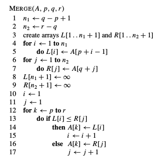
The key operation in merge sort, or any divide-and-conquer algorithm, is merging two sorted subsequences in the "combine" step. The function MERGE\((A,p,q,r)\), where \(A\) is an array and \(p\), \(q\), and \(r\) are indices numbering elements in \(A\) such that \(p \leqslant q < r\). The procedures assumes the subarrays \(A[p..q]\) and \(A[q+1..r]\) are in sorted order. It merges them to form a single sorted subarray that replaces the current subarray \(A[p..r]\). The MERGE procedure takes time \(\Theta (n)\), where \(n=r-p+1\) is how many elements are merged.
The pseudocode in Figure 3 implements MERGE, but with an additional twist that avoids having to check whether either pile is empty in each basic step. The idea is to put under each pile a sentinel card that contains a special value which causes the algorithm to terminate. Here, we use \( \infty \) as the sentinel value. When a card with \( \infty \) is exposed, it cannot be the smaller card. Since we know in advance that ALL the cards were placed in the output pile, exactly \(r-p+1\), once the sentinel card is reached. The algorithm can end.
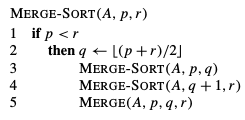
Figure 2.4 shows the pseudocode for the complete MERGE-SORT algorithm. The procedure MERGE-SORT\( ( A, p, r)\) sorts the elements in the subarray \(A[ p . . r]\). If \(p \geqslant r\), the subarray has at most one element and is therefore
already sorted. Otherwise, the divide step simply computes an index \(q\) that partitions \(A[ p..r]\) into two subarrays: \(A[ p . . q]\), containing \(\lceil n/2 \rceil\) elements, and \(A[q + 1 . . r]\), containing \(\lfloor n/2 \rfloor\) elements.
Analyzing divide-and-conquer algorithms
A recursive algorithm's running time is often described by as a recurrence equation or recurrence. Where the overall running time for a problem with size \(n\) is \(T(n)\). For a small problem size, say \(n \leqslant c\) for some constant \(c\), the solution takes a constant time written as \(\Theta(1)\).
For example, applying Merge Sort to a problem with \(n\) elements yields \(a\) subproblems. Each subproblem has the size \(n/(1/b)\). For Merge Sort \(a=b=2\). But there are many divide-and-conquer algorithms where \(a \ne b\). If creating the subproblems takes \(D(n)\) and combining the subsolutions into a solution takes \(C(n)\), the recurrence $$ T(n) = \left\{\begin{matrix} \Theta(1) & \text{if } n \leqslant c,\\ aT(n/b) + D(n)+C(n)& \text{ otherwise}\end{matrix}\right.$$ is produced.
Analyzing Merge-Sort
The pseudocode for Merge-Sort in Figures 3 and 4 works correctly with odd or even numbered elements, but a recurrence-based analysis is simplified if we assume the element count is a power of 2. Then, each divide step yields two subsequences with exactly \(n/2\) size.
The worst-case running running time for Merge-Sort on \(n\) numbers is called \(T(n)\). Sorting just one element takes constant time. With \(n > 1\) elements, the running time breaks down as follows.
Divide: The divide step into two equal subarrays takes constant time. Thus, \(D(n)= \Theta(1)\).
Conquer: Recursively solve two subproblems, each with \(n/2\) size that contributes \(2T(n/2)\) to the running time.
Combine: Note the MERGE procedure on an \(n\)-element subarray takes time \(\Theta(n)\), thus \(C(n)=\Theta(n)\).
Adding the functions \(D(n)\) and \(C(n)\) is actually adding the functions \(\Theta(n)\) and \(\Theta(1)\). This sum is a linear function for \(n\), that is, \(\Theta(n)\). Adding it to the \(2T(n/2)\) term from the "Conquer" step produces the recurrence for the worst-case running time. $$ T(n) = \left\{\begin{matrix} \Theta(1) & \text{if } n =1, & (1)\\ 2T(n/2) + \Theta(n)& \text{if } n>1. & \end{matrix}\right.$$ Later this description will be expanded to show that \(T(n)\) is \(\Theta(n \lg n)\), where \(\lg n\) stands for \(\log_{2}n\). Because the logarithm function grows more slowly than any linear function, for large enough inputs, Merge-Sort outperforms Insertion-Sort as \(\Theta(n \lg n) < \Theta(n^{2})\) in the worst case.
Describing why \(T(n) = \Theta(n \lg n) \) in another way, let's rewrite recurrence (1) as
$$ T(n) = \left\{\begin{matrix} c & \text{if } n =1, & (2)\\ 2T(n/2) + cn& \text{if } n>1. & \end{matrix}\right.$$
where the constant \(c\) represents the time required to solve problems with size 1 and the time per array element for the divide and combine steps. In real examples it is unlikely that one constant exactly represents both the time to solve problems with size 1 and the time per array element for the divide an combine steps. Here, the larger number is used and understood as the lower bounds.
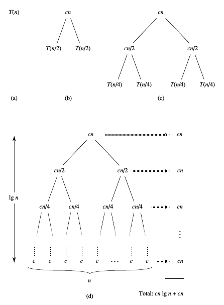
A recursion tree for recurrence (2). Part (a) show \(T(n)\), which is progressively expanded in (b)-(d) to form the recursion tree. The full tree in part (d) has \(\lg n+1\) level (i.e., it has height \(\lg n\)), and each level contributes a total cost \(cn\). The total cost is \(cn \lg n+cn\), which is \(\Theta(n \lg n)\).
Figure 5 shows how recurrence (2) can be solved. For simplicity, assume that \(n\) is an exact power of 2. Part (a) shows \(T(n)\), which in Part (b) is expanded into an equivalent tree representing the recurrence. The \(cn\) term is the root, the cost at the recursion's top level, and the two subtrees below are the smaller recurrences \(T(n/2)\). Part (c) shows the next step by expanding \(T(n/2)\). The cost for creating each subnode at the second level is \(cn/2\). The recurrence continues breaking it down into subtrees until each has the size 1 that costs \(c\). Part (d) shows the resulting tree.
Totaling the cost across each tree level proceeds as so. The top level has total cost \(cn\), the next level down costs \(c(n/2)+c(n/2)=cn\), the next level down below that costs \(c(n/4)+c(n/4)+c(n/4)+c(n/4)=cn\), and so on. In general, the \(i\)th level below the top has \(2^{i}\) nodes, each contributing a cost equal to \(c(n/2^{i})\). The \(i\)th level below the top has the total cost \(2^{i}c(n/2^{i})=cn\). The bottom level has \(n\) nodes with cost \(c\) each for a total cost \(cn\).
There are \(\lg n + 1\) levels in the recursion tree in Figure 5. This is true for all Merge-Sort trees and is easily proven by an informal inductive argument. The base case occurs when \(n=1\), in which case there is only one level. Since \(\lg 1 = 0\), we have that \(\lg n+1\) produces the correct level count. Now assume as an inductive hypothesis that the levels for a recursion tree for \(2^{i}\) nodes is \(\lg 2^{i} +1 = i+1\). Since for any value \(i\), we have that \(\lg 2^{i}=i\). Because we are assuming that the original input size is a power of 2, the next input size to consider is \(2^{i+1}\). A tree with \(2^{i+1}\) nodes has one more level than a tree with \(2^{i}\) nodes, and so the total level count is \((i+1)+1=\lg 2^{i+1}+1\).
To compute the total cost for recurrence 2 sum the costs for all levels. There are \(\lg n-1\) levels, each costing \(cn\), for a total cost \(cn(\lg n+1) = cn \lg n + cn\). Ignoring the lower-order term and the constant \(c\) produces the desired result \(\Theta (n \lg n) \).
p.36/59 2nd
Problem 2-1.
Internal Links
Parent Article: Algorithms (Advanced)(Course)
