Calculus II 06.03 Separating Variables and the Logistic Equation
| Previous | Calculus II 06.02 Differential Equations Growth and Decay |
| Next | Calculus II 06.04 First-Order Linear Differential Equations |
Contents
6.3 Separating Variables and the Logistic Equation
- Recognize and solve differential equations that can be solved by separating variables
- Use differential equations to model and solve applied problems
- Solve and analyze logistic differential equations
Separating Variables
Consider a differential equation that can be written in the form
- $$M(x)+N(y)\frac{dy}{dx}=0 $$
where \(M\) is a continuous function for \(x\) alone and \(N\) is a continuous function for \(y\) alone. All the \(x\) terms can be grouped with \(dx\) and all the \(y\) terms with \(dy\), then a solution can be obtained by integration. Such equations are said to be separable, and the solution procedure is called separation of variables. Below are some differential equations that are separable.
| Original Differential Equation | Rewritten with Variables Separated |
|---|---|
| \(x^{2}+3y{dy}{dx}=0 \) | \(3y\:dy=-x^{2}\:dx \) |
| \((\sin x)y^{\prime}=\cos x \) | \(dy=\cot x \:dx \) |
| $$\frac{xy^{\prime}}{e^{y}+1}=2 $$ | $$\frac{1}{e^{y}+1}dy=\frac{2}{x}dx $$ |
Definition 6.3.1 Separating Variables
Separating Variables is an analytical method for solving separable, first-order, differential equations. Where,
- All the \(y\) terms, including \(dy\), can be moved to one side.
- All the \(x\) terms, including \(dx\), to the other side.
The Method has three steps:
- Move all the \(y\) terms (including \(dy\) to one side and all the \(x\) terms (including \(dx\) to the other side.
- Integrate one side with respect to \(y\) and the other side with respect to \(x\). Don't forget \(+ C\) (the integration constant).
- Simplify
| Separable Multiply both sides by \(dx\). |
Non Separable Both variables are in the same function. |
| \(\frac{dy}{dx}=ky\) | \(2xy\:dx+(x^{2}-y^{2})\:dy=0\) |
The general form is \(M(x)+N(y)\frac{dy}{dx}=0\). Which solves as follows:
| \(M(x)+N(y)\frac{dy}{dx}=0\) | Original equation |
| \(M(x)\:dx+N(y)\:dy=0 \:\:\:\: \) | Multiply both sides by \(dx\) |
| \(M(x)\:dx=-N(y)\:dy\) | Subtract \(N(y)\:dy\) from both sides, the equation is separated |
Example 6.3.1 Separating Variables
Find the general solution for
- $$\frac{dy}{dx}=ky$$
Solution
1. Separate the variables across the equal sign.
| \(dy = ky \: dx\) | Multiply both sides by \(dx\) |
| $$\frac{dy}{y}=k \: dx $$ | Divide both sides by \(y\) |
2. Integrate both sides
| $$\int\frac{1}{y}\:dy=\int k\:dx $$ |
| \(\ln(y) + C_{1} = kx + C_{2}\) |
3. Simplify
| \(\ln(y) = kx+C\) |
| \(y=e^{kx+a}\) |
| \(y=e^{kx}e^{C}\) |
This form is turns up in Section 6.2 and in many, many real world examples.
Example 6.3.2 A More Complex Example
Find the general solution for
- $$y^{\prime }=\frac{2x}{y} $$
Solution
| \(y^{\prime }=\frac{2x}{y}\) | Original differential equation |
| \(y^{\prime }y=2x\) | Multiply both sides by \(y\) to ‘separate’ the \(x\)’s and the \(y\)’s. Which side each goes on is immaterial. |
| \(\int y^{\prime }ydx=\int 2x\:dx\) | Integrate BOTH sides with respect to x. |
| \(\int y\:dy = \int 2x\:dx\) | Since \(dy/dx = y^{\prime }\) substitute dy/dx for \(y^{\prime }\). |
| \(\frac{1}{2}y^{2}+C_{1}=\frac{1}{2}2x^{2}+C_{2} \:\:\:\: \) | Apply the Power Rule |
| \(\frac{1}{2}y^{2}=x^{2}+C_{2}-C_{1}\) | Simplify - Move C's to the \(x\) side. |
| \(\frac{1}{2}y^{2}=x^{2}+C\) | Simplify - \(C_{2}-C_{1} = C\) |
| \(y^{2}-2x^{2} = C\) | Simplify - Multiply both sides by 2. The new \(C\) is still \(C\). |
Example 6.3.3 Separating Variables with Multiple Solutions
Find the general solution for
- $$(x^{2}+4)\frac{dy}{dx}=xy$$
Solution Note that \(y=0\) is a solution. To find other solutions, assume that \(y \ne 0\) and separate the variables.
| \( (x^{2}+4)\:dy \) | \(=xy \: dx \) | Differential form |
| $$ \frac{dy}{y} $$ | $$= \frac{x}{x^{2}+4}dx \:\:\:\:$$ | Separate variables |
Integrate to produce the solution
| $$ \int \frac{dy}{y} $$ | $$=\int \frac{x}{x^{2}+4}dx \:\:\:\: $$ | Integrate |
| $$ \ln | y | $$ | $$ = \frac{1}{2} \ln(x^{2}+4) + C_{1} $$ | |
| \( \ln | y | \) | $$ \ln \sqrt{x^{2}+4} + C_{1} $$ | |
| \( | y | \) | $$ e^{C_{1}} \sqrt{x^{2}+4} $$ | |
| \( y \) | \( \pm e^{C_{1}} \sqrt{x^{2}+4} \) | |
| \( y \) | \( = C \sqrt{x^{2}+4} \) | The general solution |
Example 6.3.4 Finding a Particular Solution
Given the initial condition \(y(0) = 1\), find the particular solution for the equation
- \(xy\:dx+e^{-x^{2}}(y^{2}-1)\:dy=0\)
Solution Note that \(y = 0\) is a solution for the differential equation — but this solution does not satisfy the initial condition. Assume that \(y\neq 0\). Separate variables by removing \(y\) from the first term and \(e^{-x^{2}}\) from the second. Multiply both sides by \(e^{x^{2}}/y\) to produce the following.
| \(xy\:dx+e^{-x^{2}}(y^{2}-1)\:dy\) | \(=0 \) |
| \(e^{-x^{2}}(y^{2}-1)\:dy\) | \(= -xy\:dx\) |
| $$\int \left( y-\frac{1}{y} \right )\:dy $$ | $$=\int -xe^{x^{2}}\:dx $$ |
| $$\frac{y^{2}}{2}-\ln|y| $$ | $$= -\frac{1}{2}e^{x^{2}}+C$$ |
From the initial condition \(y(0) = 1\), substituting 0 for \(x\) and 1 for \(y\), produces
- $$\frac{1}{2}-0=-\frac{1}{2}+C $$
which yields \(C = 1\). The particular solution has the form
| $$\frac{y^{2}}{2}-\ln |y| $$ | $$=-\frac{1}{2}e^{x^{2}}+1 $$ |
| \(y^{2}-\ln\:y^{2}+e^{x^{2}} \) | \(=2\) |
Example 6.3.5 Finding a Particular Solution Curve
|
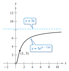
Find the equation for the curve that passes through the point \((1,3)\) and has the slope \(y/x^{2}\) at any point \((x,y)\).
with the initial condition \(y(1)=3\). Separating variables and integrating produces
Because \(y=3\) when \(x=1\), it follows that \(x=Ce^{-1}\) and \(C=3e\). The equation for the curve is
Because the solution is not defined at \(x=0\) and the initial condition is given at \(x=1\), \(x\) is restricted to positive values. See Figure 6.3.1. |
Applications
Example 6.3.6 Wildlife Population
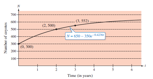
The change rate for a coyote population \(N(t)\) is directly proportional to \(650 - N(t)\), where \(t\) is time in years. When \(t=0\), the population is 300, and when \(t=2\), the population is 500. Find the population when \(t=3\).
Solution Because the change rate is proportional to \(650 - N(t)\), or \(650 - N\), the differential equation is
- $$ \frac{dN}{dt}=k(650-N) $$
Separating the variables produces.
| \(dN\) | \( =k(650-N)\:dt\) | Differential form |
| $$\frac{dn}{650-N} $$ | $$=k\:dt \:\:\:\: $$ | Separate Variables |
| \(-\ln | 650 | - N \) | \(= kt + C_{1} \:\:\:\: \) | Integrate |
| \(\ln | 650 | - N \) | \(= -kt - C_{1} \:\:\:\: \) | |
| \( 650-N \) | \(=e^{-kt-C_{1}} \) | Assume \(N < 650\) |
| \( N \) | \(=650-Ce^{-kt} \) | General Solution |
Plug in \(N=300\) when \(t=0\) produces
| \(300\) | \(=650-Ce^{-k0} \) | \(N =300\) and \(t=0\) |
| \(300\) | \(=650-C \) | |
| \(C\) | \(=350 \) |
Plug \(C=350\) into the general solution
- \(N=650-350e^{-kt}\)
Using \(N=500\) when \(t=2\), yields
- \(500=650-350e^{-2k}\:\rightarrow\:e^{-2k}=\frac{3}{7}\:\rightarrow \:k\approx 0.4236\)
The model for the coyote population is
- \(N=650-350e^{-0.4236(3)} \:\:\:\: \) Model for Population
When \(t=3\), the approximate population is
- \(N=650-350e^{-0.4236t}\approx 552\)coyotes
The model is described graphically in Figure 6.3.2. Note that \(N=650\) is the horizontal asymptote for the graph and is the carrying capacity for the model.
Orthogonal Trajectories
|
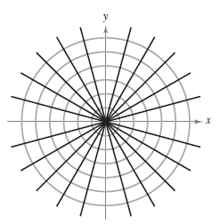
A common problem in electrostatics, thermodynamics, and hydrodynamics involves finding a curve set where each curve is orthogonal[1] to all curves in a second curve set. For example, Figure 6.3.3 shows a circle set and a line set
each circle intersects the lines in this line set
at right angles. Both curve sets are mutually orthogonal, each curve in one set is called an orthogonal trajectory to each line in the line set. In electrostatics, force lines are orthogonal to the equipotential curves. In thermodynamics, the heat flow across a plane surface is orthogonal to the isothermal curves. In hydrodynamics, the flow (stream) lines are orthogonal trajectories of the velocity potential curves. |
Example 6.3.7 Finding Orthogonal Trajectories
|
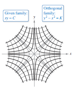
Describe the orthogonal trajectories for the inverse curve set given by
for \(C\neq 0\). Sketch the inverse curve set for several integers.
Because \(dy/dx\) represents the slop for the inverse curve set at \((x,y)\), if follow that the orthogonal curve set has the negative reciprocal slope \(x/y\). This produces
The orthogonal inverse circle set is found by separating variables and integrating.
The centers are at the origin, and the transverse axes are vertical for \(K > 0\) and horizontal for \(K \neq 0\). When \(K = 0\), the orthogonal trajectories are the lines \(y = \pm x\). When \(K \neq 0\), the orthogonal trajectories are hyperbolas. Several trajectories are shown in Figure 6.3.4. |
Logistic Differential Equation
|
In Section 6.2, the exponential growth model was derived from the fact that the change rate for a variable \(y\) is proportional to the value for \(y\). The differential equation \(dy/dt=ky\) has the general solution \(y=Ce^{kt}\). Exponential growth is unlimited, but when describing a population, there often exists some upper limit \(L\) past which growth cannot occur. This upper limit is called the carrying capacity, which is the maximum population \(y(t)\) that can be sustained or supported as time \(t\) increases. A model that is often used to describe this growth is the logistic differential equation
|
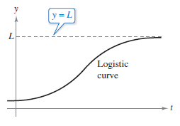
From the equation, you can see that if \(y\) is between 0 and the carrying capacity \(L\), then \(dy/dt > 0\), and the population increases. If \(y\) is greater than \(L\), then \(dy/dt < 0\), and the population decreases. The graph for function \(y\) is called the logistic curve, as shown in Figure 6.3.5.
Example 6.3.8 Deriving the General Solution
Solve the logistic differential equation
- $$\frac{dy}{dt}=ky \left (1-\frac{y}{L} \right ) \:\:\:\: \color{red}{ \text{ Logistic Differential Equation }}$$
Solution Begin by separating the variables.
| $$ \frac{dy}{dt} $$ | $$=ky \left (1-\frac{y}{L} \right ) $$ | Original Equation |
| $$ \frac{1}{y(1-y/L)}dy $$ | \(=k\:dt \) | Separate Variables |
| $$ \int \frac{1}{y(1-y/L)}dy $$ | \(=\int k\:dt \) | Integrate Both Sides |
| $$ \int \left ( \frac{1}{y} +\frac{1}{L-y} \right )dy $$ | \( =\int k\:dt\) | Rewrite Left Side using Partial Fractions |
| $$ \ln\left | y \right |-\ln\left | L-y \right | $$ | \( =kt+C\) | Find antiderivative for both sides |
| $$ \ln \left | \frac{L-y}{y} \right | $$ | \(=-kt-C\) | Multiply each side by -1 and simplify. |
| $$\left | \frac{L-y}{y} \right | $$ | \(=e^{-kt-C}\) | Exponentiate each side. |
| $$\left | \frac{L-y}{y} \right | $$ | \(=e^{-C}e^{-kt}\) | Property of Exponents |
| $$ \frac{L-y}{y} $$ | \(= be^{-kt}\) | Let \(\pm e^{-C}=b\) |
Solving this equation for \(y\) produces
- $$ y=\frac{L}{1+be^{-kt}} $$
which is the form for all logistic differential equations.
Example 6.3.9 Solving a Logistic Differential Equation
|
A state game commission releases 40 elk into a game refuge. After 5 years, the elk population is 104. The commission believes that the environment can support no more than 4000 elk. The elk population's growth rate \(p\) is
in \(t\) years.
Solution
Because \(p\)(0) = 40, you can solve for \(b\) as follows.
Then, because \(p\)=104 when \(t\)=5, you can solve for \(k\).
A model for the elk population is
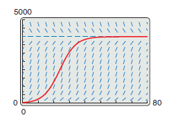
b. Using a graphing utility, you can graph the slope field for
and the solution that passes through (0,40) as shown in Figure 6.3.6.
d. As \(t\) increases without bound, the denominator
gets closer to 1. Producing
|
Internal Links
Parent Article: Calculus II 06 Differential Equations
